Reinforcement learning at Ubisoft Singapore
- Ubisoft Singapore
- Jan 26, 2021
- 7 min read
Disclaimer: An interest in the Deep Q-network (DQN) is needed for the following core concepts presented.
Video games have long proven to be fertile ground for training Artificial Intelligence (AI) with their fast-paced complex simulated environments as compared to their human counterparts in real world training situations. AI programs OpenAI Five and AlphaStar have beat the world’s best players at Dota 2 and Starcraft and the relationship between AI academic research and video games has shown that self-play Reinforcement Learning (RL) can lead to superhuman performance even on difficult tasks. The next step for the video game industry? To reverse the perspective, and to go from ‘improving RL algorithms using video games’ to ‘improving video games using RL’.
The next step for the video game industry? To reverse the perspective, and to go from ‘improving RL algorithms using video games’ to ‘improving video games using RL’.
Several Ubisoft studios are already working on this question with great success, as reflected in a new algorithm published in an academic paper from the Ubisoft Singapore team at ICML 2020 (International Conference on Machine Learning). The goal of this algorithm aims to improve how RL models are used, especially when there are many things to model at once.
Introduction to Reinforcement learning
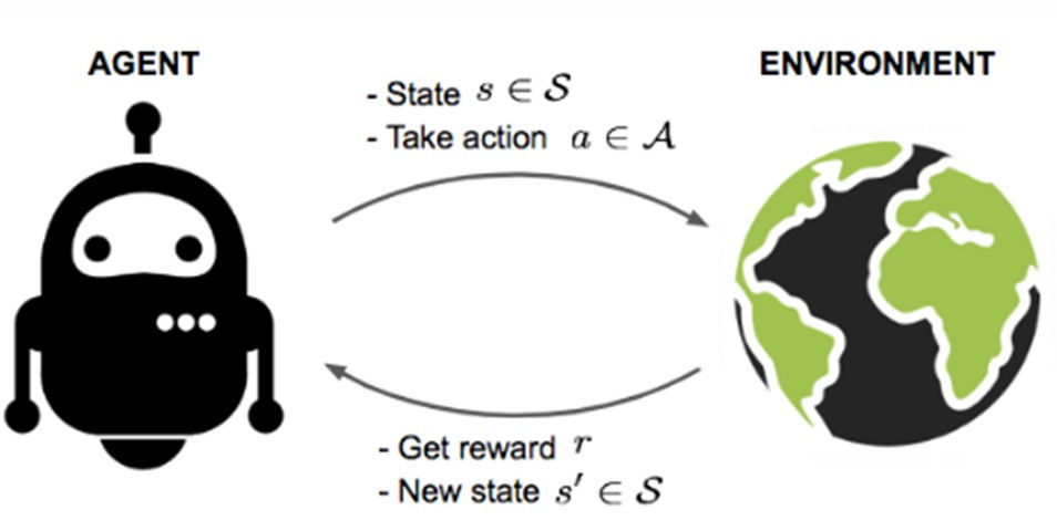
Our definition of RL is a learning framework in which an agent aims to learn the optimal way to achieve a task without any predefined logic such as a navigation mesh, and only through repeated interactions with its environment. These interactions mean collecting observations (called the ‘state’, s) from the environment, choosing an action a to perform based on this state, and receiving a reward r based on the outcome of this action in the environment. This feedback loop is represented in Figure 1 below.

Figure 1.
For instance, every n seconds, an agent driving a vehicle collects information about the environment (speed, direction, surroundings), before deciding whether it should turn, accelerate or brake. If it crashes, it gets penalized with a negative reward.
Based on this interaction loop, the agent attempts to maximize the discounted rewards it receives at each timestep. We say discounted as it reflects that the agent would rather have an immediate positive reward instead of waiting several timesteps to get it. Intuitively, it’s expected that the agent will avoid actions yielding negative rewards and favor the positive ones. Since rewards are directly linked to the success of the task, the agent will thus learn how to achieve the task in an optimal way, without the need to hardcode logic.
Q-Learning algorithm
A successful method to learn the optimal sequence of actions, based on the state of the environment, is Q-learning. It uses a specific function, called the Q-function. This tells the agent what reward to expect for a given state s, if it executes action a, followed by an optimal sequence of actions. The agent can then achieve the optimal behavior (or optimal policy) by choosing at each timestep, the action a associated with the highest Q-function value (or Q-value). The agent best succeeds if it learns the Q-value for each state and action combination. As it interacts with the environment, it updates the Q-values using new learnings with the following algorithm in Figure 2.

There are different ways to represent the Q-function. If the number of states and action is small, we can represent it in a tabular way. However, in most cases the dimension of the state space is huge and it cannot do so.
The solution is to use a function approximator, like a neural network, to represent the Q-function. This solves computational issues as the number of parameters needed to represent the Q-function is reduced. This algorithm is called ‘Deep Q-Network’ (DQN) – a mix between Deep Learning (i.e. neural networks) and Q-learning!
Using DQN with continuous actions: a complexity challenge.
The DQN algorithm was originally designed to handle discrete actions (i.e. an action which can take only a limited number of values) as represented in the Q-learning update rule (see Figure 2.).
One needs to take the maximum value of the Q-function over all the action a’ available in state s’. When the set of possible actions is finite, the hint used in the DQN algorithm is to have the last layer of the neural network outputting the Q value for all possible actions and then selecting the maximum value. It is not possible with continuous actions since the last layer of the network cannot have an infinite dimension.
Several algorithms were developed to directly handle continuous action spaces, such as Deep Deterministic Policy Gradient (DDPG) or Soft Actor-Critic (SAC). However, these methods have their own flaws and it is sometimes better to stick to the DQN algorithm even with continuous action spaces. The trick mostly used is to discretize the continuous action space into n different bins, that cover the whole space. Thanks to this transformation, the action space is now made up of n discrete actions, with which one can use with the DQN algorithm.
Nonetheless, another issue arises when the agent needs to choose several different actions (called sub-actions in the rest of the article) at the same time. Using again our car navigation example, at each second t, an agent needs to choose to steer the wheels from x degrees (sub-action 1, noted s1) while accelerating by y m/s with the throttle (sub-action 2, s2) and using the brake at z percent (sub-action 3, s3). The final action space is the cartesian product of all these sub-actions spaces. It means that if one discretizes each sub-action space into n bins, the final action space has n x n x n = n3 possible discrete action tuples (s1, s2, s3) among which one needs to choose the maximum. With m sub-actions and n discrete bins for each, the number of possible discrete action tuples is nm, a number which grows exponentially with the number of sub-actions. Once again there is a computational issue.
A solution is to decompose the Q network into m sub-modules, each of them being responsible to choose one sub-action (see Figure 3.2). As a result, instead of having a single huge network which takes as input the state s and has nm output values, one has m different sub network which take as input the state s and have n output values respectively. Thus, the maximum is only taken over n values m times, so we have n x m operations.
The problem is that we now assume that each sub-action is independent from the other ones, which was not the case with the vanilla architecture. Indeed, each action sub module has no information about the other sub-actions selected by the other sub-modules. It is possible to solve this issue by using a fully sequential structure (see Figure 3.3), where each action sub-module takes as input the state s and the sub-actions already chosen by the sub-modules ‘higher’ in the structure, and outputs n values, over which one takes the argmax to pass to the next sub-module in the hierarchy. This structure models dependences between each sub-action, but the ordering of the sub-modules (i.e. which sub-module should one put on top, who will have the less information available, which sub-module needs more information and should be put lower in the structure) is left to the practitioner.
In the paper published, our team at Ubisoft Singapore proposed a new method to infer this structure from uncertainty measurements.

Figure 3.
Introducing ordering in the network architecture: the uncertainty measure.
The main idea developed is for the ordering of the sub-modules to be based on the uncertainty associated to these modules during the learning phase. Sub-modules exhibiting high uncertainty during the learning phase, when trained with the fully parallel architecture (i.e. with no information from the other sub-modules), would benefit from having more information coming from other more certain modules, and thus should be placed ‘lower’ in the sequential structure. Based on this, the following training method is proposed to infer the structure of the neural network (see Figure 4).

Figure 4.
In our method, we tested two different methods to estimate uncertainty. We focused on the epistemic uncertainty, which is the one that comes from the lack of agent’s knowledge and can be reduced by interacting more with the environment and collecting more data (as opposed to the aleatoric uncertainty which comes from the randomness in the environment itself and cannot be reduced).
Since tackling the problem of reducing epistemic uncertainty is tightly linked with exploring efficiently the environment, the first method we devised uses a former technique developed initially to foster better exploration behavior, called Noisy DQN. The idea is to model the weights of the Q-network not as variable parameters you can optimize but instead as random variables, defined by their mean and standard deviation. It means that when the network is trained, we do not directly optimize the weights of the network but instead their means and standard deviations. In this setup, we used the standard deviation of the weights as a measure of uncertainty: if the weights have a standard deviation which moves a lot, it means that the network is highly uncertain about the weights.
The second method to infer an uncertainty measure for each sub-module that we tried is to directly use the output values of each sub-module. For a given state s, if the sub-module is certain which action it should select, then one Q-value would be higher than the others, meaning a high standard deviation among the output values. On the contrary, if the sub-module is uncertain about which action to choose, it will output similar values for all sub-actions, so the standard deviation will be low.
Results and next steps
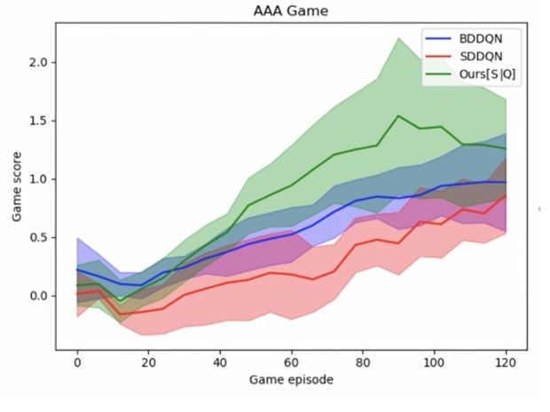
Most of our tests were carried out in Mujoco, a standard environment to simulate physics movements. The various goals being to a human leg model (‘Hopper’), human lower body model (‘Walker’), a dog model (‘Cheetah’) and a full human model (‘Humanoid’) to walk with each of them being made up of several actuators controlling joints. As we represented each of these actuators as action sub-modules and applied our novel technique on it, we could achieve state of the arts results on these toy examples hence the decision to bring this technique into ship navigation. In that framework, the action sub-modules were the different parameters one can tweak in the game to control the ship, i.e. the sail rotation angle, the steering wheel rotation angle and the sail opening. It’s all pretty exciting stuff if you ask us.

At Ubisoft, we apply Reinforcement Learning in a multitude of ways but there is always more to be learned and applied. Not only in Singapore but in our other studios as well, we’re excited to continually build upon what has been done. Think you’re up for a good challenge in the world of building AAA blockbuster games? Check out our job openings here, you might just be the right fit for we’re looking for.

Comments